Let x be a discrete random variable. Actions on events

Purpose of the service. The online calculator is used to construct a table of the distribution of the random variable X - the number of experiments performed and to calculate all the characteristics of the series: mathematical expectation, dispersion and standard deviation. The report with the decision is drawn up in Word format.

Example 1. In the urn white and black ball. Balls are drawn at random from the urn without returning until a white ball appears. As soon as this happens, the process stops.
This type of task relates to the problem of constructing a geometric distribution.

Example 2. Two Three shooters each fire one shot at the target. The probability of the first shooter hitting it is , second –

. Draw up a distribution law for the random variable X - the number of hits on the target. , Example 2a. The shooter fires two three four shots. The probability of hitting with a corresponding shot is equal to

. If the first miss occurs, the shooter does not participate in further competitions. Draw up a distribution law for the random variable X - the number of hits on the target. Example 3. In the party from details defective standard ones. The controller draws at random
details. Draw up a distribution law for the random variable X - the number of defective good parts in the sample. Similar task
: There are m red and n blue balls in the basket. K balls are drawn at random. Draw up the law of distribution of DSV X - the appearance of blue balls.

see other example solutions. Example 4. The probability of an event occurring in one trial is equal to . Produced
tests. Draw up a law of distribution of the random variable X - the number of occurrences of the event.:
Similar tasks for this type of distribution
1. Draw up a distribution law for the random variable X number of hits with four shots, if the probability of hitting the target with one shot is 0.8.

js-script
Example No. 1. Three coins are tossed. The probability of getting a coat of arms in one throw is 0.5. Draw up a distribution law for the random variable X - the number of dropped emblems.
Solution.
Probability that no coat of arms was drawn: P(0) = 0.5*0.5*0.5= 0.125 0,5 *0,5*0,5 + 0,5*0,5 *0,5 + 0,5*0,5*0,5 = 3*0,125=0,375
P(1) = 0,5 *0,5 *0,5 + 0,5 *0,5*0,5 + 0,5*0,5 *0,5 = 3*0,125=0,375
P(2) =

Distribution law of random variable X:

X	0	1	2	3
P	0,125	0,375	0,375	0,125

Check: P = P(0) + P(1) + P(2) + P(3) = 0.125 + 0.375 + 0.375 + 0.125 = 1

Example No. 2. The probability of one shooter hitting the target with one shot for the first shooter is 0.8, for the second shooter – 0.85. The shooters fired one shot at the target. Considering hitting the target as independent events for individual shooters, find the probability of event A – exactly one hit on the target.
Example No. 1. Three coins are tossed. The probability of getting a coat of arms in one throw is 0.5. Draw up a distribution law for the random variable X - the number of dropped emblems.
Consider event A - one hit on the target. Possible options for this event to occur are as follows:

1. The first shooter hit, the second shooter missed: P(A/H1)=p 1 *(1-p 2)=0.8*(1-0.85)=0.12
2. The first shooter missed, the second shooter hit the target: P(A/H2)=(1-p 1)*p 2 =(1-0.8)*0.85=0.17
3. The first and second arrows hit the target independently of each other: P(A/H1H2)=p 1 *p 2 =0.8*0.85=0.68

Then the probability of event A – exactly one hit on the target – will be equal to: P(A) = 0.12+0.17+0.68 = 0.97

X; meaning F(5); the probability that the random variable X will take values ​​from the segment . Construct a distribution polygon.

1. The distribution function F(x) of a discrete random variable is known X:

Set the law of distribution of a random variable X in the form of a table.

1. The law of distribution of a random variable is given X:

X	–28	–20	–12	–4
p	0,22	0,44	0,17	0,1	0,07

1. The probability that the store has quality certificates for the full range of products is 0.7. The commission checked the availability of certificates in four stores in the area. Draw up a distribution law, calculate the mathematical expectation and dispersion of the number of stores in which quality certificates were not found during inspection.

1. To determine the average burning time of electric lamps in a batch of 350 identical boxes, one electric lamp from each box was taken for testing. Estimate from below the probability that the average burning duration of the selected electric lamps differs from the average burning duration of the entire batch in absolute value by less than 7 hours, if it is known that the standard deviation of the burning duration of electric lamps in each box is less than 9 hours.

1. At a telephone exchange, an incorrect connection occurs with a probability of 0.002. Find the probability that among 500 connections the following will occur:

Find the distribution function of a random variable X. Construct graphs of functions and . Calculate the mathematical expectation, variance, mode and median of a random variable X.

1. An automatic machine makes rollers. It is believed that their diameter is a normally distributed random variable with a mean value of 10 mm. What is the standard deviation if, with a probability of 0.99, the diameter is in the range from 9.7 mm to 10.3 mm.

Sample A: 6 9 7 6 4 4

Sample B: 55 72 54 53 64 53 59 48

42 46 50 63 71 56 54 59

54 44 50 43 51 52 60 43

50 70 68 59 53 58 62 49

59 51 52 47 57 71 60 46

55 58 72 47 60 65 63 63

58 56 55 51 64 54 54 63

56 44 73 41 68 54 48 52

52 50 55 49 71 67 58 46

50 51 72 63 64 48 47 55

Option 17.

1. Among the 35 parts, 7 are non-standard. Find the probability that two parts taken at random will turn out to be standard.

1. Three dice are thrown. Find the probability that the sum of points on the dropped sides is a multiple of 9.

1. The word “ADVENTURE” is made up of cards, each with one letter written on it. The cards are shuffled and taken out one at a time without returning. Find the probability that the letters taken out in the order of appearance form the word: a) ADVENTURE; b) PRISONER.

1. An urn contains 6 black and 5 white balls. 5 balls are randomly drawn. Find the probability that among them there are:
1. 2 white balls;
2. less than 2 white balls;
3. at least one black ball.

1. A in one test is equal to 0.4. Find the probabilities of the following events:
1. event A appears 3 times in a series of 7 independent trials;
2. event A will appear no less than 220 and no more than 235 times in a series of 400 trials.

1. The plant sent 5,000 good-quality products to the base. The probability of damage to each product in transit is 0.002. Find the probability that no more than 3 products will be damaged during the journey.

1. The first urn contains 4 white and 9 black balls, and the second urn contains 7 white and 3 black balls. 3 balls are randomly drawn from the first urn, and 4 from the second urn. Find the probability that all the drawn balls are the same color.

1. The law of distribution of a random variable is given X:

Calculate its mathematical expectation and variance.

1. There are 10 pencils in the box. 4 pencils are drawn at random. Random value X– the number of blue pencils among those selected. Find the law of its distribution, the initial and central moments of the 2nd and 3rd orders.

1. The technical control department checks 475 products for defects. The probability that the product is defective is 0.05. Find, with probability 0.95, the boundaries within which the number of defective products among those tested will be contained.

1. At a telephone exchange, an incorrect connection occurs with a probability of 0.003. Find the probability that among 1000 connections the following will occur:
1. at least 4 incorrect connections;
2. more than two incorrect connections.

1. The random variable is specified by the distribution density function:

Find the distribution function of a random variable X. Construct graphs of functions and . Calculate the mathematical expectation, variance, mode and median of the random variable X.

1. The random variable is specified by the distribution function:

1. By sample A solve the following problems:
1. create a variation series;

· sample average;

· sample variance;

Mode and median;

Sample A: 0 0 2 2 1 4

1. calculate the numerical characteristics of the variation series:

· sample average;

· sample variance;

standard sample deviation;

· mode and median;

Sample B: 166 154 168 169 178 182 169 159

161 150 149 173 173 156 164 169

157 148 169 149 157 171 154 152

164 157 177 155 167 169 175 166

167 150 156 162 170 167 161 158

168 164 170 172 173 157 157 162

156 150 154 163 143 170 170 168

151 174 155 163 166 173 162 182

166 163 170 173 159 149 172 176

Option 18.

1. Among 10 lottery tickets, 2 are winning ones. Find the probability that out of five tickets taken at random, one will be a winner.

1. Three dice are thrown. Find the probability that the sum of the rolled points is greater than 15.

1. The word “PERIMETER” is made up of cards, each of which has one letter written on it. The cards are shuffled and taken out one at a time without returning. Find the probability that the letters taken out form the word: a) PERIMETER; b) METER.

1. An urn contains 5 black and 7 white balls. 5 balls are randomly drawn. Find the probability that among them there are:
1. 4 white balls;
2. less than 2 white balls;
3. at least one black ball.

1. Probability of an event occurring A in one trial is equal to 0.55. Find the probabilities of the following events:
1. event A will appear 3 times in a series of 5 challenges;
2. event A will appear no less than 130 and no more than 200 times in a series of 300 trials.

1. The probability of a can of canned goods breaking is 0.0005. Find the probability that among 2000 cans, two will have a leak.

1. The first urn contains 4 white and 8 black balls, and the second urn contains 7 white and 4 black balls. Two balls are randomly drawn from the first urn and three balls are randomly drawn from the second urn. Find the probability that all the drawn balls are the same color.

1. Among the parts arriving for assembly, 0.1% are defective from the first machine, 0.2% from the second, 0.25% from the third, and 0.5% from the fourth. The machine productivity ratios are respectively 4:3:2:1. The part taken at random turned out to be standard. Find the probability that the part was made on the first machine.

1. The law of distribution of a random variable is given X:

Calculate its mathematical expectation and variance.

1. An electrician has three light bulbs, each of which has a defect with a probability of 0.1. The light bulbs are screwed into the socket and the current is turned on. When the current is turned on, the defective light bulb immediately burns out and is replaced by another. Find the distribution law, mathematical expectation and dispersion of the number of tested light bulbs.

1. The probability of hitting a target is 0.3 for each of 900 independent shots. Using Chebyshev's inequality, estimate the probability that the target will be hit at least 240 times and at most 300 times.

1. At a telephone exchange, an incorrect connection occurs with a probability of 0.002. Find the probability that among 800 connections the following will occur:
1. at least three incorrect connections;
2. more than four incorrect connections.

1. The random variable is specified by the distribution density function:

Find the distribution function of the random variable X. Draw graphs of the functions and . Calculate the mathematical expectation, variance, mode and median of a random variable X.

1. The random variable is specified by the distribution function:

1. By sample A solve the following problems:
1. create a variation series;
2. calculate relative and accumulated frequencies;
3. compile an empirical distribution function and plot it;
4. calculate the numerical characteristics of the variation series:

· sample average;

· sample variance;

standard sample deviation;

· mode and median;

Sample A: 4 7 6 3 3 4

1. Using sample B, solve the following problems:
1. create a grouped variation series;
2. build a histogram and frequency polygon;
3. calculate the numerical characteristics of the variation series:

· sample average;

· sample variance;

standard sample deviation;

· mode and median;

Sample B: 152 161 141 155 171 160 150 157

154 164 138 172 155 152 177 160

168 157 115 128 154 149 150 141

172 154 144 177 151 128 150 147

143 164 156 145 156 170 171 142

148 153 152 170 142 153 162 128

150 146 155 154 163 142 171 138

128 158 140 160 144 150 162 151

163 157 177 127 141 160 160 142

159 147 142 122 155 144 170 177

Option 19.

1. There are 16 women and 5 men working at the site. 3 people were selected at random using their personnel numbers. Find the probability that all selected people will be men.

2. Four coins are tossed. Find the probability that only two coins will have a “coat of arms”.

3. The word “PSYCHOLOGY” is made up of cards, each of which has one letter written on it. The cards are shuffled and taken out one at a time without returning. Find the probability that the letters taken out form a word: a) PSYCHOLOGY; b) STAFF.

4. The urn contains 6 black and 7 white balls. 5 balls are randomly drawn. Find the probability that among them there are:

a. 3 white balls;

b. less than 3 white balls;

c. at least one white ball.

5. Probability of an event occurring A in one trial is equal to 0.5. Find the probabilities of the following events:

a. event A appears 3 times in a series of 5 independent trials;

b. event A will appear at least 30 and no more than 40 times in a series of 50 trials.

6. There are 100 machines of the same power, operating independently of each other in the same mode, in which their drive is turned on for 0.8 working hours. What is the probability that at any given moment in time from 70 to 86 machines will be turned on?

7. The first urn contains 4 white and 7 black balls, and the second urn contains 8 white and 3 black balls. 4 balls are randomly drawn from the first urn, and 1 ball from the second. Find the probability that among the drawn balls there are only 4 black balls.

8. The car sales showroom receives cars of three brands daily in volumes: “Moskvich” – 40%; "Oka" - 20%; "Volga" - 40% of all imported cars. Among Moskvich cars, 0.5% have an anti-theft device, Oka – 0.01%, Volga – 0.1%. Find the probability that the car taken for inspection has an anti-theft device.

9. Numbers and are chosen at random on the segment. Find the probability that these numbers satisfy the inequalities.

10. The law of distribution of a random variable is given X:

X
p	0,1	0,2	0,3	0,4

Find the distribution function of a random variable X; meaning F(2); the probability that the random variable X will take values ​​from the interval . Construct a distribution polygon.

Random variable A variable is called a variable that, as a result of each test, takes on one previously unknown value, depending on random reasons. Random variables are denoted by capital Latin letters: $X,\ Y,\ Z,\ \dots $ According to their type, random variables can be discrete And continuous.

Discrete random variable- this is a random variable whose values ​​can be no more than countable, that is, either finite or countable. By countability we mean that the values ​​of a random variable can be numbered.

Example 1 . Here are examples of discrete random variables:

a) the number of hits on the target with $n$ shots, here the possible values ​​are $0,\ 1,\ \dots ,\ n$.

b) the number of emblems dropped when tossing a coin, here the possible values ​​are $0,\ 1,\ \dots ,\ n$.

c) the number of ships arriving on board (a countable set of values).

d) the number of calls arriving at the PBX (countable set of values).

1. Law of probability distribution of a discrete random variable.

A discrete random variable $X$ can take values ​​$x_1,\dots ,\ x_n$ with probabilities $p\left(x_1\right),\ \dots ,\ p\left(x_n\right)$. The correspondence between these values ​​and their probabilities is called law of distribution of a discrete random variable. As a rule, this correspondence is specified using a table, the first line of which indicates the values ​​$x_1,\dots ,\ x_n$, and the second line contains the probabilities $p_1,\dots ,\ p_n$ corresponding to these values.

$\begin(array)(|c|c|)
\hline
X_i & x_1 & x_2 & \dots & x_n \\
\hline
p_i & p_1 & p_2 & \dots & p_n \\
\hline
\end(array)$

Example 2 . Let the random variable $X$ be the number of points rolled when tossing a die. Such a random variable $X$ can take the following values: $1,\ 2,\ 3,\ 4,\ 5,\ 6$. The probabilities of all these values ​​are equal to $1/6$. Then the law of probability distribution of the random variable $X$:

$\begin(array)(|c|c|)
\hline
1 & 2 & 3 & 4 & 5 & 6 \\
\hline

\hline
\end(array)$

Comment. Since in the distribution law of a discrete random variable $X$ the events $1,\ 2,\ \dots ,\ 6$ form a complete group of events, then the sum of the probabilities must be equal to one, that is, $\sum(p_i)=1$.

2. Mathematical expectation of a discrete random variable.

Expectation of a random variable sets its “central” meaning. For a discrete random variable, the mathematical expectation is calculated as the sum of the products of the values ​​$x_1,\dots ,\ x_n$ and the probabilities $p_1,\dots ,\ p_n$ corresponding to these values, that is: $M\left(X\right)=\sum ^n_(i=1)(p_ix_i)$. In English-language literature, another notation $E\left(X\right)$ is used.

Properties of mathematical expectation$M\left(X\right)$:

1. $M\left(X\right)$ lies between the smallest and largest values ​​of the random variable $X$.
2. The mathematical expectation of a constant is equal to the constant itself, i.e. $M\left(C\right)=C$.
3. The constant factor can be taken out of the sign of the mathematical expectation: $M\left(CX\right)=CM\left(X\right)$.
4. The mathematical expectation of the sum of random variables is equal to the sum of their mathematical expectations: $M\left(X+Y\right)=M\left(X\right)+M\left(Y\right)$.
5. The mathematical expectation of the product of independent random variables is equal to the product of their mathematical expectations: $M\left(XY\right)=M\left(X\right)M\left(Y\right)$.

Example 3 . Let's find the mathematical expectation of the random variable $X$ from example $2$.

$$M\left(X\right)=\sum^n_(i=1)(p_ix_i)=1\cdot ((1)\over (6))+2\cdot ((1)\over (6) )+3\cdot ((1)\over (6))+4\cdot ((1)\over (6))+5\cdot ((1)\over (6))+6\cdot ((1 )\over (6))=3.5.$$

We can notice that $M\left(X\right)$ lies between the smallest ($1$) and largest ($6$) values ​​of the random variable $X$.

Example 4 . It is known that the mathematical expectation of the random variable $X$ is equal to $M\left(X\right)=2$. Find the mathematical expectation of the random variable $3X+5$.

Using the above properties, we get $M\left(3X+5\right)=M\left(3X\right)+M\left(5\right)=3M\left(X\right)+5=3\cdot 2 +5=11$.

Example 5 . It is known that the mathematical expectation of the random variable $X$ is equal to $M\left(X\right)=4$. Find the mathematical expectation of the random variable $2X-9$.

Using the above properties, we get $M\left(2X-9\right)=M\left(2X\right)-M\left(9\right)=2M\left(X\right)-9=2\cdot 4 -9=-1$.

3. Dispersion of a discrete random variable.

Possible values ​​of random variables with equal mathematical expectations can disperse differently around their average values. For example, in two student groups the average score for the exam in probability theory turned out to be 4, but in one group everyone turned out to be good students, and in the other group there were only C students and excellent students. Therefore, there is a need for a numerical characteristic of a random variable that would show the spread of the values ​​of the random variable around its mathematical expectation. This characteristic is dispersion.

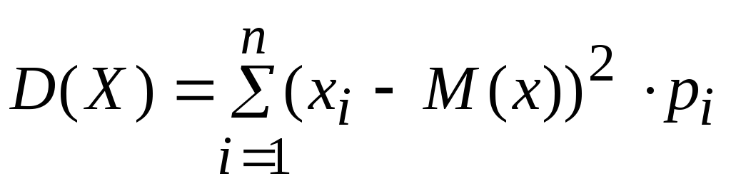
Variance of a discrete random variable$X$ is equal to:

$$D\left(X\right)=\sum^n_(i=1)(p_i(\left(x_i-M\left(X\right)\right))^2).\ $$

In English literature the notation $V\left(X\right),\ Var\left(X\right)$ is used. Very often the variance $D\left(X\right)$ is calculated using the formula $D\left(X\right)=\sum^n_(i=1)(p_ix^2_i)-(\left(M\left(X \right)\right))^2$.

Dispersion properties$D\left(X\right)$:

1. The variance is always greater than or equal to zero, i.e. $D\left(X\right)\ge 0$.
2. The variance of the constant is zero, i.e. $D\left(C\right)=0$.
3. The constant factor can be taken out of the sign of the dispersion provided that it is squared, i.e. $D\left(CX\right)=C^2D\left(X\right)$.
4. The variance of the sum of independent random variables is equal to the sum of their variances, i.e. $D\left(X+Y\right)=D\left(X\right)+D\left(Y\right)$.
5. The variance of the difference between independent random variables is equal to the sum of their variances, i.e. $D\left(X-Y\right)=D\left(X\right)+D\left(Y\right)$.

Example 6 . Let's calculate the variance of the random variable $X$ from example $2$.

$$D\left(X\right)=\sum^n_(i=1)(p_i(\left(x_i-M\left(X\right)\right))^2)=((1)\over (6))\cdot (\left(1-3.5\right))^2+((1)\over (6))\cdot (\left(2-3.5\right))^2+ \dots +((1)\over (6))\cdot (\left(6-3.5\right))^2=((35)\over (12))\approx 2.92.$$

Example 7 . It is known that the variance of the random variable $X$ is equal to $D\left(X\right)=2$. Find the variance of the random variable $4X+1$.

Using the above properties, we find $D\left(4X+1\right)=D\left(4X\right)+D\left(1\right)=4^2D\left(X\right)+0=16D\ left(X\right)=16\cdot 2=32$.

Example 8 . It is known that the variance of the random variable $X$ is equal to $D\left(X\right)=3$. Find the variance of the random variable $3-2X$.

Using the above properties, we find $D\left(3-2X\right)=D\left(3\right)+D\left(2X\right)=0+2^2D\left(X\right)=4D\ left(X\right)=4\cdot 3=12$.

4. Distribution function of a discrete random variable.

The method of representing a discrete random variable in the form of a distribution series is not the only one, and most importantly, it is not universal, since a continuous random variable cannot be specified using a distribution series. There is another way to represent a random variable - the distribution function.

Distribution function random variable $X$ is called a function $F\left(x\right)$, which determines the probability that the random variable $X$ will take a value less than some fixed value $x$, that is, $F\left(x\right )=P\left(X< x\right)$

Properties of the distribution function:

1. $0\le F\left(x\right)\le 1$.
2. The probability that the random variable $X$ will take values ​​from the interval $\left(\alpha ;\ \beta \right)$ is equal to the difference between the values ​​of the distribution function at the ends of this interval: $P\left(\alpha< X < \beta \right)=F\left(\beta \right)-F\left(\alpha \right)$
3. $F\left(x\right)$ - non-decreasing.
4. $(\mathop(lim)_(x\to -\infty ) F\left(x\right)=0\ ),\ (\mathop(lim)_(x\to +\infty ) F\left(x \right)=1\ )$.

Example 9 . Let us find the distribution function $F\left(x\right)$ for the distribution law of the discrete random variable $X$ from example $2$.

$\begin(array)(|c|c|)
\hline
1 & 2 & 3 & 4 & 5 & 6 \\
\hline
1/6 & 1/6 & 1/6 & 1/6 & 1/6 & 1/6 \\
\hline
\end(array)$

If $x\le 1$, then, obviously, $F\left(x\right)=0$ (including for $x=1$ $F\left(1\right)=P\left(X< 1\right)=0$).

If $1< x\le 2$, то $F\left(x\right)=P\left(X=1\right)=1/6$.

If $2< x\le 3$, то $F\left(x\right)=P\left(X=1\right)+P\left(X=2\right)=1/6+1/6=1/3$.

If $3< x\le 4$, то $F\left(x\right)=P\left(X=1\right)+P\left(X=2\right)+P\left(X=3\right)=1/6+1/6+1/6=1/2$.

If $4< x\le 5$, то $F\left(X\right)=P\left(X=1\right)+P\left(X=2\right)+P\left(X=3\right)+P\left(X=4\right)=1/6+1/6+1/6+1/6=2/3$.

If $5< x\le 6$, то $F\left(x\right)=P\left(X=1\right)+P\left(X=2\right)+P\left(X=3\right)+P\left(X=4\right)+P\left(X=5\right)=1/6+1/6+1/6+1/6+1/6=5/6$.

If $x > 6$, then $F\left(x\right)=P\left(X=1\right)+P\left(X=2\right)+P\left(X=3\right) +P\left(X=4\right)+P\left(X=5\right)+P\left(X=6\right)=1/6+1/6+1/6+1/6+ 1/6+1/6=1$.

So $F(x)=\left\(\begin(matrix)
0,\ at\ x\le 1,\\
1/6,at\ 1< x\le 2,\\
1/3,\ at\ 2< x\le 3,\\
1/2,at\ 3< x\le 4,\\
2/3,\ at\ 4< x\le 5,\\
5/6,\ at\ 4< x\le 5,\\
1,\ for\ x > 6.
\end(matrix)\right.$

Definition 2.3. A random variable, denoted by X, is called discrete if it takes on a finite or countable set of values, i.e. set – a finite or countable set.

Let's consider examples of discrete random variables.

1. Two coins are tossed once. The number of emblems in this experiment is a random variable X. Its possible values ​​are 0,1,2, i.e. – a finite set.

2. The number of ambulance calls within a given period of time is recorded. Random value X– number of calls. Its possible values ​​are 0, 1, 2, 3, ..., i.e. =(0,1,2,3,...) is a countable set.

3. There are 25 students in the group. On a certain day, the number of students who came to class is recorded - a random variable X. Its possible values: 0, 1, 2, 3, ...,25 i.e. =(0, 1, 2, 3, ..., 25).

Although all 25 people in example 3 cannot miss classes, the random variable X can take this value. This means that the values ​​of a random variable have different probabilities.

Let's consider a mathematical model of a discrete random variable.

Let a random experiment be carried out, which corresponds to a finite or countable space of elementary events. Let us consider the mapping of this space onto the set of real numbers, i.e., let us assign to each elementary event a certain real number , . The set of numbers can be finite or countable, i.e. or

A system of subsets, which includes any subset, including a one-point one, forms an -algebra of a numerical set ( – finite or countable).

Since any elementary event is associated with certain probabilities p i(in the case of finite everything), and , then each value of a random variable can be associated with a certain probability p i, such that .

Let X is an arbitrary real number. Let's denote R X (x) the probability that the random variable X took a value equal to X, i.e. P X (x)=P(X=x). Then the function R X (x) can take positive values ​​only for those values X, which belong to a finite or countable set , and for all other values ​​the probability of this value P X (x)=0.

So, we have defined the set of values, -algebra as a system of any subsets and for each event ( X = x) compared the probability for any, i.e. constructed a probability space.

For example, the space of elementary events of an experiment consisting of tossing a symmetrical coin twice consists of four elementary events: , where

When the coin was tossed twice, two tails appeared; when the coin was tossed twice, two coats of arms fell;

On the first toss of the coin, a hash came up, and on the second, a coat of arms;

On the first toss of the coin, the coat of arms came up, and on the second, the hash mark.

Let the random variable X– number of grating dropouts. It is defined on and the set of its values . All possible subsets, including single-point ones, form an algebra, i.e. =(Ø, (1), (2), (0,1), (0,2), (1,2), (0,1,2)).

Probability of an event ( X=x i}, і = 1,2,3, we define as the probability of the occurrence of an event that is its prototype:

Thus, on elementary events ( X = x i) set a numerical function R X, So .

Definition 2.4. The law of distribution of a discrete random variable is a set of pairs of numbers (x i, р i), where x i are the possible values ​​of the random variable, and р i are the probabilities with which it takes these values, and .

The simplest form of specifying the distribution law of a discrete random variable is a table that lists the possible values ​​of the random variable and the corresponding probabilities:

			…		…
			…		…

Such a table is called a distribution series. To give the distribution series a more visual appearance, it is depicted graphically: on the axis Oh dots x i and draw perpendiculars of length from them p i. The resulting points are connected and a polygon is obtained, which is one of the forms of the distribution law (Fig. 2.1).

Thus, to specify a discrete random variable, you need to specify its values ​​and the corresponding probabilities.

Example 2.2. The cash slot of the machine is triggered each time a coin is inserted with the probability R. Once it is triggered, the coins do not come down. Let X– the number of coins that must be inserted before the machine’s cash slot is triggered. Construct a series of distribution of a discrete random variable X.

Example No. 1. Three coins are tossed. The probability of getting a coat of arms in one throw is 0.5. Draw up a distribution law for the random variable X - the number of dropped emblems. Possible values ​​of a random variable X: x 1 = 1, x 2 = 2,..., x k = k, ... Let's find the probabilities of these values: p 1– the probability that the money receiver will operate the first time it is lowered, and p 1 = p; p 2 – the probability that two attempts will be made. To do this, it is necessary that: 1) the money receiver does not work on the first attempt; 2) on the second try it worked. The probability of this event is (1–р)р. Likewise and so on, . Distribution range X will take the form

	1	2	3	…	To	…
	R	qp	q 2 p		q r -1 p

Note that the probabilities r k form a geometric progression with the denominator: 1–p=q, q<1, therefore this probability distribution is called geometric.

Let us further assume that a mathematical model has been constructed experiment described by a discrete random variable X, and consider calculating the probabilities of the occurrence of arbitrary events.

Let an arbitrary event contain a finite or countable set of values x i: A= {x 1, x 2,..., x i, ...) .Event A can be represented as a union of incompatible events of the form: . Then, using Kolmogorov’s axiom 3 , we get

since we determined the probabilities of the occurrence of events to be equal to the probabilities of the occurrence of events that are their prototypes. This means that the probability of any event , , can be calculated using the formula, since this event can be represented in the form of a union of events, where .

Then the distribution function F(x) = Р(–<Х<х) is found by the formula. It follows that the distribution function of a discrete random variable X is discontinuous and increases in jumps, i.e. it is a step function (Fig. 2.2):

If the set is finite, then the number of terms in the formula is finite, but if it is countable, then the number of terms is countable.

Example 2.3. The technical device consists of two elements that operate independently of each other. The probability of failure of the first element during time T is 0.2, and the probability of failure of the second element is 0.1. Random value X– the number of failed elements during time T. Find the distribution function of the random variable and plot its graph.

Example No. 1. Three coins are tossed. The probability of getting a coat of arms in one throw is 0.5. Draw up a distribution law for the random variable X - the number of dropped emblems. The space of elementary events of an experiment consisting of studying the reliability of two elements of a technical device is determined by four elementary events , , , : – both elements are operational; – the first element is working, the second is faulty; – the first element is faulty, the second is working; – both elements are faulty. Each of the elementary events can be expressed through elementary events of spaces And , where – the first element is operational; – the first element has failed; – the second element is working; – the second element has failed. Then, and since the elements of a technical device work independently of each other, then

8. What is the probability that the values ​​of a discrete random variable belong to the interval?

In applications of probability theory, the quantitative characteristics of the experiment are of primary importance. A quantity that can be quantitatively determined and which, as a result of an experiment, can take on different values ​​depending on the case is called random variable.

Examples of random variables:

1. The number of times an even number of points appears in ten throws of a die.

2. The number of hits on the target by a shooter who fires a series of shots.

3. The number of fragments of an exploding shell.

In each of the examples given, the random variable can only take on isolated values, that is, values ​​that can be numbered using a natural series of numbers.

Such a random variable, the possible values ​​of which are individual isolated numbers, which this variable takes with certain probabilities, is called discrete.

The number of possible values ​​of a discrete random variable can be finite or infinite (countable).

Law of distribution A discrete random variable is a list of its possible values ​​and their corresponding probabilities. The distribution law of a discrete random variable can be specified in the form of a table (probability distribution series), analytically and graphically (probability distribution polygon).

When carrying out an experiment, it becomes necessary to evaluate the value being studied “on average.” The role of the average value of a random variable is played by a numerical characteristic called mathematical expectation, which is determined by the formula

Where x 1 , x 2 ,.. , x n– random variable values X, A p 1 ,p 2 , ... , p n– the probabilities of these values ​​(note that p 1 + p 2 +…+ p n = 1).

Example. Shooting is carried out at the target (Fig. 11).

A hit in I gives three points, in II – two points, in III – one point. The number of points scored in one shot by one shooter has a distribution law of the form

To compare the skill of shooters, it is enough to compare the average values ​​of the points scored, i.e. mathematical expectations M(X) And M(Y):

M(X) = 1 0,4 + 2  0,2 + 3  0,4 = 2,0,

M(Y) = 1 0,2 + 2  0,5 + 3  0,3 = 2,1.

The second shooter gives on average a slightly higher number of points, i.e. it will give better results when fired repeatedly.

Let us note the properties of the mathematical expectation:

1. The mathematical expectation of a constant value is equal to the constant itself:

M(C) = C.

2. The mathematical expectation of the sum of random variables is equal to the sum of the mathematical expectations of the terms:

M =(X 1 + X 2 +…+ X n)= M(X 1)+ M(X 2)+…+ M(X n).

3. The mathematical expectation of the product of mutually independent random variables is equal to the product of the mathematical expectations of the factors

M(X 1 X 2 … X n) = M(X 1)M(X 2)… M(X n).

4. The mathematical negation of the binomial distribution is equal to the product of the number of trials and the probability of an event occurring in one trial (task 4.6).

M(X) = pr.

To assess how a random variable “on average” deviates from its mathematical expectation, i.e. In order to characterize the spread of values ​​of a random variable in probability theory, the concept of dispersion is used.

Variance random variable X is called the mathematical expectation of the squared deviation:

D(X) = M[(X - M(X)) 2 ].

Dispersion is a numerical characteristic of the dispersion of a random variable. From the definition it is clear that the smaller the dispersion of a random variable, the more closely its possible values ​​are located around the mathematical expectation, that is, the better the values ​​of the random variable are characterized by its mathematical expectation.

From the definition it follows that the variance can be calculated using the formula

.

It is convenient to calculate the variance using another formula:

D(X) = M(X 2) - (M(X)) 2 .

The dispersion has the following properties:

1. The variance of the constant is zero:

D(C) = 0.

2. The constant factor can be taken out of the dispersion sign by squaring it:

D(CX) = C 2 D(X).

3. The variance of the sum of independent random variables is equal to the sum of the variance of the terms:

D(X 1 + X 2 + X 3 +…+ X n)= D(X 1)+ D(X 2)+…+ D(X n)

4. The variance of the binomial distribution is equal to the product of the number of trials and the probability of the occurrence and non-occurrence of an event in one trial:

D(X) = npq.

In probability theory, a numerical characteristic equal to the square root of the variance of a random variable is often used. This numerical characteristic is called the mean square deviation and is denoted by the symbol

.

It characterizes the approximate size of the deviation of a random variable from its average value and has the same dimension as the random variable.

4.1. The shooter fires three shots at the target. The probability of hitting the target with each shot is 0.3.

Construct a distribution series for the number of hits.

Solution. The number of hits is a discrete random variable X. Each value x n random variable X corresponds to a certain probability P n .

The distribution law of a discrete random variable in this case can be specified near distribution.

In this problem X takes values ​​0, 1, 2, 3. According to Bernoulli's formula

,

Let's find the probabilities of possible values ​​of the random variable:

R 3 (0) = (0,7) 3 = 0,343,

R 3 (1) =0,3(0,7) 2 = 0,441,

R 3 (2) =(0,3) 2 0,7 = 0,189,

R 3 (3) = (0,3) 3 = 0,027.

By arranging the values ​​of the random variable X in increasing order, we obtain the distribution series:

X n

Note that the amount

means the probability that the random variable X will take at least one value from among the possible ones, and this event is reliable, therefore

.

4.2 .There are four balls in the urn with numbers from 1 to 4. Two balls are taken out. Random value X– the sum of the ball numbers. Construct a distribution series of a random variable X.

Example No. 1. Three coins are tossed. The probability of getting a coat of arms in one throw is 0.5. Draw up a distribution law for the random variable X - the number of dropped emblems. Random variable values X are 3, 4, 5, 6, 7. Let's find the corresponding probabilities. Random variable value 3 X can be accepted in the only case when one of the selected balls has the number 1, and the other 2. The number of possible test outcomes is equal to the number of combinations of four (the number of possible pairs of balls) of two.

Using the classical probability formula we get

Likewise,

R(X= 4) =R(X= 6) =R(X= 7) = 1/6.

The sum 5 can appear in two cases: 1 + 4 and 2 + 3, so

.

X has the form:

Find the distribution function F(x) random variable X and plot it. Calculate for X its mathematical expectation and variance.

Solution. The distribution law of a random variable can be specified by the distribution function

F(x) =P(X x).

Distribution function F(x) is a non-decreasing, left-continuous function defined on the entire number line, while

F (- )= 0,F (+ )= 1.

For a discrete random variable, this function is expressed by the formula

.

Therefore in this case

Distribution function graph F(x) is a stepped line (Fig. 12)

	F(x)

Expected valueM(X) is the weighted arithmetic average of the values X 1 , X 2 ,……X n random variable X with scales ρ 1, ρ 2, …… , ρ n and is called the mean value of the random variable X. According to the formula

M(X)= x 1 ρ 1 + x 2 ρ 2 +……+ x n ρ n

M(X) = 3·0.14+5·0.2+7·0.49+11·0.17 = 6.72.

Dispersion characterizes the degree of dispersion of the values ​​of a random variable from its average value and is denoted D(X):

D(X)=M[(HM(X)) 2 ]= M(X 2) –[M(X)] 2 .

For a discrete random variable, the variance has the form

or it can be calculated using the formula

Substituting the numerical data of the problem into the formula, we get:

M(X 2) = 3 2 ∙ 0,14+5 2 ∙ 0,2+7 2 ∙ 0,49+11 2 ∙ 0,17 = 50,84

D(X) = 50,84-6,72 2 = 5,6816.

4.4. Two dice are rolled twice at the same time. Write the binomial law of distribution of a discrete random variable X- the number of occurrences of an even total number of points on two dice.

Solution. Let us introduce a random event

A= (two dice with one throw resulted in a total of even number of points).

Using the classical definition of probability we find

R(A)= ,

Where n - the number of possible test outcomes is found according to the rule

multiplication:

n = 6∙6 =36,

m - number of people favoring the event A outcomes - equal

m= 3∙6=18.

Thus, the probability of success in one trial is

ρ = P(A)= 1/2.

The problem is solved using a Bernoulli test scheme. One challenge here will be rolling two dice once. Number of such tests n = 2. Random variable X takes values ​​0, 1, 2 with probabilities

R 2 (0) =,R 2 (1) =∙,R 2 (2) =

The desired binomial distribution of a random variable X can be represented as a distribution series:

X n
ρ n

4.5 . In a batch of six parts there are four standard ones. Three parts were selected at random. Construct a probability distribution of a discrete random variable X– the number of standard parts among those selected and find its mathematical expectation.

Example No. 1. Three coins are tossed. The probability of getting a coat of arms in one throw is 0.5. Draw up a distribution law for the random variable X - the number of dropped emblems. Random variable values X are the numbers 0,1,2,3. It's clear that R(X=0)=0, since there are only two non-standard parts.

R(X=1) =
=1/5,

R(X= 2) =
= 3/5,

R(X=3) =
= 1/5.

Distribution law of a random variable X Let's present it in the form of a distribution series:

X n
ρ n

Expected value

M(X)=1 ∙ 1/5+2 ∙ 3/5+3 ∙ 1/5=2.

4.6 . Prove that the mathematical expectation of a discrete random variable X- number of occurrences of the event A V n independent trials, in each of which the probability of an event occurring is equal to ρ – equal to the product of the number of trials by the probability of the occurrence of an event in one trial, that is, to prove that the mathematical expectation of the binomial distribution

M(X) =n . ρ ,

and dispersion

D(X) =n.p. .

Example No. 1. Three coins are tossed. The probability of getting a coat of arms in one throw is 0.5. Draw up a distribution law for the random variable X - the number of dropped emblems. Random value X can take values ​​0, 1, 2..., n. Probability R(X= k) is found using Bernoulli’s formula:

R(X=k)= R n(k)= ρ To (1-ρ ) n- To

Distribution series of a random variable X has the form:

X n
ρ n	q n	ρq n- 1	ρq n- 2		ρ n

Where q= 1- ρ .

For the mathematical expectation we have the expression:

M(X)=ρq n - 1 +2 ρ 2 q n - 2 +…+.n ρ n

In the case of one test, that is, with n= 1 for random variable X 1 – number of occurrences of the event A- the distribution series has the form:

X n
ρ n

M(X 1)= 0∙q + 1 ∙ p = p

D(X 1) = p – p 2 = p(1- p) = pq.

If X k – number of occurrences of the event A in which test, then R(X To)= ρ And

X=X 1 +X 2 +….+X n .

From here we get

M(X)=M(X 1 )+M(X 2)+ … +M(X n)= nρ,

D(X)=D(X 1)+D(X 2)+ ... +D(X n)=npq.

4.7. The quality control department checks products for standardness. The probability that the product is standard is 0.9. Each batch contains 5 products. Find the mathematical expectation of a discrete random variable X- the number of batches, each of which will contain 4 standard products - if 50 batches are subject to inspection.

Solution. The probability that there will be 4 standard products in each randomly selected batch is constant; let's denote it by ρ .Then the mathematical expectation of the random variable X equals M(X)= 50∙ρ.

Let's find the probability ρ according to Bernoulli's formula:

ρ=P 5 (4)== 0,94∙0,1=0,32.

M(X)= 50∙0,32=16.

4.8 . Three dice are thrown. Find the mathematical expectation of the sum of the dropped points.

Example No. 1. Three coins are tossed. The probability of getting a coat of arms in one throw is 0.5. Draw up a distribution law for the random variable X - the number of dropped emblems. You can find the distribution of a random variable X- the sum of the dropped points and then its mathematical expectation. However, this path is too cumbersome. It is easier to use another technique, representing a random variable X, the mathematical expectation of which needs to be calculated, in the form of a sum of several simpler random variables, the mathematical expectation of which is easier to calculate. If the random variable X i is the number of points rolled on i– th bones ( i= 1, 2, 3), then the sum of points X will be expressed in the form

X = X 1 + X 2 + X 3 .

To calculate the mathematical expectation of the original random variable, all that remains is to use the property of mathematical expectation

M(X 1 + X 2 + X 3 )= M(X 1 )+ M(X 2)+ M(X 3 ).

It's obvious that

R(X i = K)= 1/6, TO= 1, 2, 3, 4, 5, 6, i= 1, 2, 3.

Therefore, the mathematical expectation of the random variable X i looks like

M(X i) = 1/6∙1 + 1/6∙2 +1/6∙3 + 1/6∙4 + 1/6∙5 + 1/6∙6 = 7/2,

M(X) = 3∙7/2 = 10,5.

4.9. Determine the mathematical expectation of the number of devices that failed during testing if:

a) the probability of failure for all devices is the same R, and the number of devices under test is equal to n;

b) probability of failure for i – of the device is equal to p i , i= 1, 2, … , n.

Example No. 1. Three coins are tossed. The probability of getting a coat of arms in one throw is 0.5. Draw up a distribution law for the random variable X - the number of dropped emblems. Let the random variable X is the number of failed devices, then

X = X 1 + X 2 + … + X n ,

X i =

It's clear that

R(X i = 1)= R i , R(X i = 0)= 1– R i ,i= 1, 2, … ,n.

M(X i)= 1∙R i + 0∙(1-R i)=P i ,

M(X)=M(X 1)+M(X 2)+ … +M(X n)=P 1 +P 2 + … + P n .

In case “a” the probability of device failure is the same, that is

R i =p,i= 1, 2, … ,n.

M(X)= n.p..

This answer could be obtained immediately if we notice that the random variable X has a binomial distribution with parameters ( n, p).

4.10. Two dice are thrown simultaneously twice. Write the binomial law of distribution of a discrete random variable X - the number of rolls of an even number of points on two dice.

Solution. Let

A=(rolling an even number on the first dice),

B =(rolling an even number on the second dice).

Getting an even number on both dice in one throw is expressed by the product AB. Then

R (AB) = R(A)∙R(IN) =
.

The result of the second throw of two dice does not depend on the first, so Bernoulli's formula applies when

n = 2,p = 1/4, q = 1– p = 3/4.

Random value X can take values ​​0, 1, 2 , the probability of which can be found using Bernoulli’s formula:

R(X= 0)= P 2 (0) = q 2 = 9/16,

R(X= 1)= P 2 (1)= C ,R∙q = 6/16,

R(X= 2)= P 2 (2)= C , R 2 = 1/16.

Distribution series of a random variable X:

4.11. The device consists of a large number of independently operating elements with the same very small probability of failure of each element over time t. Find the average number of refusals over time t elements, if the probability that at least one element will fail during this time is 0.98.

Example No. 1. Three coins are tossed. The probability of getting a coat of arms in one throw is 0.5. Draw up a distribution law for the random variable X - the number of dropped emblems. Number of people who refused over time t elements – random variable X, which is distributed according to Poisson's law, since the number of elements is large, the elements work independently and the probability of failure of each element is small. Average number of occurrences of an event in n tests equals

M(X) = n.p..

Since the probability of failure TO elements from n expressed by the formula

R n (TO)
,

where  = n.p., then the probability that not a single element will fail during the time t we get at K = 0:

R n (0)= e -  .

Therefore, the probability of the opposite event is in time t at least one element fails – equal to 1 - e -  . According to the conditions of the problem, this probability is 0.98. From Eq.

1 - e -  = 0,98,

e -  = 1 – 0,98 = 0,02,

from here  = -ln 0,02  4.

So, in time t operation of the device, on average 4 elements will fail.

4.12 . The dice are rolled until a “two” comes up. Find the average number of throws.

Solution. Let's introduce a random variable X– the number of tests that must be performed until the event of interest to us occurs. The probability that X= 1 is equal to the probability that during one throw of the dice a “two” will appear, i.e.

R(X= 1) = 1/6.

Event X= 2 means that on the first test the “two” did not come up, but on the second it did. Probability of event X= 2 is found by the rule of multiplying the probabilities of independent events:

R(X= 2) = (5/6)∙(1/6)

Likewise,

R(X= 3) = (5/6) 2 ∙1/6, R(X= 4) = (5/6) 2 ∙1/6

etc. We obtain a series of probability distributions:

					(5/6) To ∙1/6

The average number of throws (trials) is the mathematical expectation

M(X) = 1∙1/6 + 2∙5/6∙1/6 + 3∙(5/6) 2 ∙1/6 + … + TO (5/6) TO -1 ∙1/6 + … =

1/6∙(1+2∙5/6 +3∙(5/6) 2 + … + TO (5/6) TO -1 + …)

Let's find the sum of the series:

TOg TO -1 = (g TO) g 
.

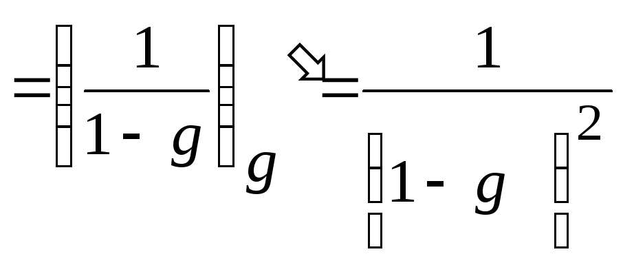Hence,

M(X) = (1/6) (1/ (1 – 5/6) 2 = 6.

Thus, you need to make an average of 6 throws of the dice until a “two” comes up.

4.13. Independent tests are carried out with the same probability of occurrence of the event A in every test. Find the probability of an event occurring A, if the variance of the number of occurrences of an event in three independent trials is 0.63 .

Example No. 1. Three coins are tossed. The probability of getting a coat of arms in one throw is 0.5. Draw up a distribution law for the random variable X - the number of dropped emblems. The number of occurrences of an event in three trials is a random variable X, distributed according to the binomial law. The variance of the number of occurrences of an event in independent trials (with the same probability of occurrence of the event in each trial) is equal to the product of the number of trials by the probabilities of the occurrence and non-occurrence of the event (problem 4.6)

D(X) = npq.

By condition n = 3, D(X) = 0.63, so you can R find from equation

0,63 = 3∙R(1-R),

which has two solutions R 1 = 0.7 and R 2 = 0,3.