The significance of the regression equation as a whole is assessed. Solution using Excel spreadsheet processor
To assess the significance and significance of the correlation coefficient, the Student's t-test is used.
The average error of the correlation coefficient is found using the formula:
N  and based on the error, the t-criterion is calculated:
The calculated t-test value is compared with the tabulated value found in the Student's distribution table at a significance level of 0.05 or 0.01 and the number of degrees of freedom n-1. If the calculated value of the t-test is greater than the table value, then the correlation coefficient is considered significant.
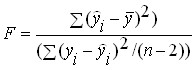
In the case of a curvilinear relationship, the F-test is used to assess the significance of the correlation relationship and the regression equation. It is calculated by the formula:

or 
where η is the correlation ratio; n – number of observations; m – number of parameters in the regression equation.
The calculated F value is compared with the tabulated one for the accepted significance level α (0.05 or 0.01) and the numbers of degrees of freedom k 1 =m-1 and k 2 =n-m. If the calculated F value exceeds the table one, the relationship is considered significant.
The significance of the regression coefficient is established using the Student t-test, which is calculated using the formula:

where σ 2 and i is the variance of the regression coefficient.
It is calculated by the formula:

where k is the number of factor characteristics in the regression equation.
The regression coefficient is considered significant if t a 1 ≥t cr.
t cr is found in the table of critical points of the Student distribution at the accepted significance level and the number of degrees of freedom k=n-1.
4.3. Correlation and regression analysis in Excel – the yield of grain crops, in cells B1:B30, the value of the resulting characteristic is the cost of labor per 1 quintal of grain. In the Tools menu, select the Data Analysis option. By left-clicking on this item, we will open the Regression tool. Click the OK button and the Regression dialog box appears on the screen. In the Input interval Y field, enter the values of the resultant characteristic (highlighting cells B1:B30), in the Input interval X field, enter the values of the factor characteristic (highlighting cells A1:A30). Mark the 95% probability level and select New Worksheet. Click on the OK button. The “CONCLUSION OF RESULTS” table appears on the worksheet, which shows the results of calculating the parameters of the regression equation, the correlation coefficient and other indicators that allow you to determine the significance of the correlation coefficient and the parameters of the regression equation.
|
CONCLUSION OF RESULTS | ||||||||
|
Regression statistics | ||||||||
|
Plural R | ||||||||
|
R-square | ||||||||
|
Normalized R-squared | ||||||||
|
Standard error | ||||||||
|
Observations | ||||||||
|
Analysis of variance | ||||||||
|
Significance F | ||||||||
|
Regression | ||||||||
|
Odds |
Standard error |
t-statistic |
P-Value |
Bottom 95% |
Top 95% |
Bottom 95.0% |
Top 95.0% |
|
|
Y-intersection | ||||||||
|
Variable X 1 | ||||||||
In this table, “Multiple R” is the correlation coefficient, “R-squared” is the coefficient of determination. “Coefficients: Y-intersection” - free term of the regression equation 2.836242; “Variable X1” – regression coefficient -0.06654. There are also values of Fisher’s F-test 74.9876, Student’s t-test 14.18042, “Standard error 0.112121”, which are necessary to assess the significance of the correlation coefficient, parameters of the regression equation and the entire equation.
Based on the data in the table, we will construct a regression equation: y x = 2.836-0.067x. The regression coefficient a 1 = -0.067 means that with an increase in grain yield by 1 c/ha, labor costs per 1 c of grain decrease by 0.067 man-hours.
The correlation coefficient is r=0.85>0.7, therefore, the relationship between the studied characteristics in this population is close. The coefficient of determination r 2 =0.73 shows that 73% of the variation in the effective trait (labor costs per 1 quintal of grain) is caused by the action of the factor trait (grain yield).
In the table of critical points of the Fisher-Snedecor distribution, we find the critical value of the F-test at a significance level of 0.05 and the number of degrees of freedom k 1 =m-1=2-1=1 and k 2 =n-m=30-2=28, it is equal to 4.21. Since the calculated value of the criterion is greater than the tabulated one (F=74.9896>4.21), the regression equation is considered significant.
To assess the significance of the correlation coefficient, let’s calculate the Student’s t-test:
IN  In the table of critical points of the Student distribution, we find the critical value of the t-test at a significance level of 0.05 and the number of degrees of freedom n-1=30-1=29, it is equal to 2.0452. Since the calculated value is greater than the table value, the correlation coefficient is significant.
For regression equation coefficients, their significance level is checked by t -Student's criterion and according to the criterion F Fisher. Below we will consider assessing the reliability of regression indicators only for linear equations (12.1) and (12.2).
Y=a 0+a 1 X(12.1)
X= b 0+b 1 Y(12.2)
For this type of equations it is estimated by t-Student's t-test only for coefficient values A 1i b 1using value calculation Tf according to the following formulas:
Where r yx correlation coefficient, and the value A 1 can be calculated using formulas 12.5 or 12.7.
Formula (12.27) is used to calculate the quantity Tf, A 1regression equations Y By X.

Size b 1 can be calculated using formulas (12.6) or (12.8).
Formula (12.29) is used to calculate the quantity Tf, which allows you to assess the significance level of the coefficient b 1regression equations X By Y
Example. Let's estimate the level of significance of the regression coefficients A 1i b 1 equations (12.17), and (12.18), obtained by solving problem 12.1. For this we use formulas (12.27), (12.28), (12.29) and (12.30).
Let us recall the form of the obtained regression equations:
Y x = 3 + 0,06 X(12.17)
X y = 9+ 1 Y(12.19)
Magnitude A 1 in equation (12.17) is equal to 0.06. Therefore, to calculate using formula (12.27), you need to calculate the value Sb y x. According to the problem conditions, the value P= 8. The correlation coefficient has also already been calculated by us using formula 12.9: r xy = √ 0,06 0,997 = 0,244 .
It remains to calculate the quantities Σ (y ι- y) 2 and Σ (X ι –x) 2, which we have not counted. These calculations are best done in Table 12.2:
Table 12.2
| No. of subjects | x ι | y i | x ι –x | (x ι –x) 2 | y ι- y | (y ι- y) 2 |
| -4,75 | 22,56 | - 1,75 | 3,06 | |||
| -4,75 | 22,56 | -0,75 | 0,56 | |||
| -2,75 | 7,56 | 0,25 | 0,06 | |||
| -2,75 | 7,56 | 1,25 | 15,62 | |||
| 1,25 | 1,56 | 1,25 | 15,62 | |||
| 3,25 | 10,56 | 0,25 | 0,06 | |||
| 5,25 | 27,56 | -0,75 | 0,56 | |||
| 5,25 | 27,56 | 0,25 | 0,06 | |||
| Amounts | 127,48 | 35,6 | ||||
| Average | 12,75 | 3,75 |
We substitute the obtained values into formula (12.28), we get:
Now let's calculate the value Tf according to formula (12.27):

Magnitude Tf is checked for significance level according to Table 16 of Appendix 1 for t- Student's t test. The number of degrees of freedom in this case will be equal to 8-2 = 6, therefore the critical values are equal respectively for P ≤ 0,05 t cr= 2.45 and for P≤ 0,01 t cr=3.71. In the accepted form of notation it looks like this:

We build the “axis of significance”:

The resulting value Tf But that the value of the regression coefficient of equation (12.17) is indistinguishable from zero. In other words, the resulting regression equation is inadequate to the original experimental data.
Let us now calculate the significance level of the coefficient b 1. To do this, it is necessary to calculate the value Sb xy according to formula (12.30), for which all the necessary quantities have already been calculated:
Now let's calculate the value Tf according to formula (12.27):

We can immediately construct a “significance axis”, since all the preliminary operations have been done above:

The resulting value Tf fell into the zone of insignificance, therefore we must accept the hypothesis H that the value of the regression coefficient of equation (12.19) is indistinguishable from zero. In other words, the resulting regression equation is inadequate to the original experimental data.
Nonlinear regression
The result obtained in the previous section is somewhat discouraging: we found that both regression equations (12.15) and (12.17) are inadequate to the experimental data. The latter happened because both of these equations characterize the linear relationship between the characteristics, and in section 11.9 we showed that between the variables X And Y there is a significant curvilinear relationship. In other words, between the variables X And Y in this problem it is necessary to look for curvilinear rather than linear connections. We will do this using the “Stage 6.0” package (developed by A.P. Kulaichev, registration number 1205).
Problem 12.2. The psychologist wants to select a regression model that is adequate to the experimental data obtained in problem 11.9.
Solution. This problem is solved by simply searching through the curvilinear regression models offered in the Stadiya statistical package. The package is organized in such a way that the experimental data is entered into the spreadsheet, which is the source for further work, in the form of the first column for the variable X and a second column for the variable Y. Then in the main menu, select the Statistics section, in it there is a subsection - regression analysis, in this subsection again a subsection - curvilinear regression. The last menu contains formulas (models) for various types of curvilinear regression, according to which you can calculate the corresponding regression coefficients and immediately check them for significance. Below we will look at just a few examples of working with ready-made curvilinear regression models (formulas).
1. First model - exponent . Its formula is:
![]()
When calculating using the statistical package, we get A 0 = 1 and A 1 = 0,022.
Calculation of the significance level for a, gave the value R= 0.535. Obviously, the resulting value is insignificant. Therefore, this regression model is inadequate to the experimental data.
2. Second model - power . Its formula is:
![]()
When counting a o = - 5.29, a, = 7.02 and A 1 = 0,0987.
Significance level for A 1 - R= 7.02 and for A 2 - P = 0.991. Obviously, none of the coefficients are significant.
3. Third model - polynomial . Its formula is:
Y= A 0 + A 1 X + a 2 X 2+ A 3 X 3
When counting a 0= - 29,8, A 1 = 7,28, A 2 = - 0.488 and A 3 = 0.0103. Significance level for a, - P = 0.143, for a 2 - P = 0.2 and for a, - P= 0,272
Conclusion - this model is inadequate to experimental data.
4. Fourth model - parabola .
Its formula is: Y= a o + a l -X 1 + a 2 X 2
When counting A 0 = - 9.88, a, = 2.24 and A 1 = - 0.0839 Significance level for A 1 - P = 0.0186, for A 2 - P = 0.0201. Both regression coefficients were significant. Consequently, the problem is solved - we have identified the form of a curvilinear relationship between the success of solving the third Wechsler subtest and the level of knowledge in algebra - this is a parabolic relationship. This result confirms the conclusion obtained when solving Problem 11.9 about the presence of a curvilinear relationship between the variables. We emphasize that it was with the help of curvilinear regression that the exact form of the relationship between the studied variables was obtained.
Chapter 13 FACTOR ANALYSIS
Basic concepts of factor analysis
Factor analysis is a statistical method that is used when processing large amounts of experimental data. The objectives of factor analysis are: reducing the number of variables (data reduction) and determining the structure of relationships between variables, i.e. classification of variables, so factor analysis is used as a data reduction method or as a structural classification method.
An important difference between factor analysis and all the methods described above is that it cannot be used to process primary, or, as they say, “raw” experimental data, i.e. obtained directly from the examination of subjects. The material for factor analysis is correlations, or more precisely, Pearson correlation coefficients, which are calculated between the variables (i.e. psychological characteristics) included in the survey. In other words, correlation matrices, or, as they are otherwise called, intercorrelation matrices, are subjected to factor analysis. The column and row names in these matrices are the same because they represent a list of variables included in the analysis. For this reason, intercorrelation matrices are always square, i.e. the number of rows in them is equal to the number of columns, and symmetrical, i.e. symmetrical places relative to the main diagonal have the same correlation coefficients.
It must be emphasized that the original data table from which the correlation matrix is obtained does not have to be square. For example, a psychologist measured three indicators of intelligence (verbal, nonverbal and general) and school grades in three academic subjects (literature, mathematics, physics) from 100 subjects - ninth grade students. The original data matrix will be 100 × 6 in size and the intercorrelation matrix will be 6 × 6 in size because there are only 6 variables. With such a number of variables, the intercorrelation matrix will include 15 coefficients and analyzing it will not be difficult.
However, imagine what will happen if the psychologist receives not 6, but 100 indicators from each subject. In this case, he will have to analyze 4950 correlation coefficients. The number of coefficients in the matrix is calculated by the formula n (n+1)/2 and in our case is equal to (100×99)/2= 4950.
Obviously, conducting a visual analysis of such a matrix is a difficult task. Instead, the psychologist can perform a mathematical procedure for factor analysis of a 100 × 100 correlation matrix (100 subjects and 100 variables) and thus obtain simpler material for interpreting experimental results.
The main concept of factor analysis is factor. This is an artificial statistical indicator that arises as a result of special transformations of the table of correlation coefficients between the studied psychological characteristics, or the intercorrelation matrix. The procedure for extracting factors from an intercorrelation matrix is called matrix factorization. As a result of factorization, a different number of factors can be extracted from the correlation matrix, up to a number equal to the number of original variables. However, the factors identified as a result of factorization, as a rule, are unequal in importance.
The elements of the factor matrix are called or scales"; and they represent the correlation coefficients of a given factor with all indicators used in the study. The factor matrix is very important because it shows how the indicators being studied are related to each selected factor. At the same time, the factor weight demonstrates the measure, or closeness, of this connection.
Since each column of the factor matrix (factor) is a kind of variable, the factors themselves can also correlate with each other. There are two possible cases here: the correlation between factors is zero, in which case the factors are independent (orthogonal). If the correlation between factors is greater than zero, then the factors are considered dependent (oblique). We emphasize that orthogonal factors, unlike oblique factors, provide simpler options for interactions within the factor matrix.
As an illustration of orthogonal factors, the problem of L. Thurstone is often cited, who, taking a number of boxes of different sizes and shapes, measured more than 20 different indicators in each of them and calculated the correlations between them. Having factorized the resulting intercorrelation matrix, he obtained three factors, the correlation between which was equal to zero. These factors were "length", "width" and "height".
In order to better grasp the essence of factor analysis, let us examine the following example in more detail.
Suppose that a psychologist obtains the following data from a random sample of students:
V 1- body weight (in kg);
V 2 - number of visits to lectures and seminars on the subject;
V 3- leg length (in cm);
V 4- number of books read on the subject;
V 5- arm length (in cm);
V 6 - examination grade in the subject ( V- from the English word variable - variable).
When analyzing these features, it is not unreasonable to assume that the variables V 1, K 3 and V 5- will be interconnected, since the larger the person, the more he weighs and the longer his limbs. This means that statistically significant correlation coefficients should be obtained between these variables because these three variables measure some fundamental property of the individuals in the sample, namely their size. It is equally likely that when calculating correlations between V 2, V 4 And V 6 Quite high correlation coefficients will also be obtained, since attending lectures and self-study will contribute to obtaining higher grades in the subject being studied.
Thus, from the entire possible array of coefficients, which is obtained by enumerating pairs of correlated features V 1 And V 2 , V t And V 3 etc., two blocks of statistically significant correlations are expected to stand out. The rest of the correlations, between traits included in different blocks, are unlikely to have statistically significant coefficients, since connections between traits such as limb size and academic performance are most likely random in nature. So, a meaningful analysis of our 6 variables shows that they, in fact, measure only two generalized characteristics, namely: body size and the degree of preparedness in the subject.
To the resulting intercorrelation matrix, i.e. calculated pairwise correlation coefficients between all six variables V 1 - V 6, It is permissible to apply factor analysis. It can be carried out manually, using a calculator, but the procedure for such statistical processing is very labor-intensive. For this reason, factor analysis is currently carried out on computers, usually using standard statistical packages. All modern statistical packages have programs for correlation and factor analysis. A factor analysis computer program essentially attempts to “explain” correlations between variables in terms of a small number of factors (two in our example).
Suppose that, using a computer program, we obtained an intercorrelation matrix of all six variables and subjected it to factor analysis. As a result of the factor analysis, Table 13.1 was obtained, which is called the “factor matrix” or “factor structural matrix”.
Table 13.1
| Variable | Factor 1 | Factor 2 |
| V 1 | 0,91 | 0,01 |
| V 2 | 0,20 | 0,96 |
| V 3 | 0,94 | -0,15 |
| V 4 | 0,11 | 0,85 |
| V 5 | 0,89 | 0,07 |
| V 6 | -0,13 | 0,93 |
Traditionally, factors are represented in a table as columns, and variables as rows. The column headings of Table 13.1 correspond to the numbers of the identified factors, but it would be more accurate to call them “factor loadings”, or “weights”, for factor 1, the same for factor 2. As stated above, factor loadings, or weights, are correlations between the corresponding variable and a given factor. For example, the first number of 0.91 in the first factor means that the correlation between the first factor and the variable V 1 equal to 0.91. The higher the factor loading in absolute value, the greater its relationship with the factor.
From Table 13.1 it can be seen that the variables V 1 V 3 And V 5 have large correlations with factor 1 (in fact, variable 3 has a correlation close to 1 with factor 1). At the same time the variables V 2 ,V 3 and U 5 have correlations close to 0 with factor 2. Similarly, factor 2 is highly correlated with the variables V 2, V 4 And V 6 and does not actually correlate with the variables V 1,V 3 and V 5
In this example, it is clear that there are two correlation structures, and therefore all of the information in Table 13.1 is determined by two factors. Now the final stage of work begins - interpretation of the data obtained. When analyzing a factor matrix, it is very important to take into account the signs of factor loadings in each factor. If there are loadings with opposite signs in the same factor, this means that there is an inversely proportional relationship between variables that have opposite signs.
Note that when interpreting a factor, for convenience, you can change the signs of all loadings on a given factor to the opposite ones.
The factor matrix also shows which variables form each factor. This is due, first of all, to the level of significance of the factor weight. Traditionally, the minimum level of significance of correlation coefficients in factor analysis is taken to be 0.4 or even 0.3 (in absolute value), since there are no special tables from which to determine the critical values for the level of significance in the factor matrix. Therefore, the easiest way to see which variables “belong” to a factor is to mark those that have loadings greater than 0.4 (or less than -0.4). We point out that in computer packages sometimes the level of significance of the factor weight is determined by the program itself and is set at a higher level, for example 0.7.
So, from table 13.1, it follows that factor 1 is a combination of variables V 1 K 3 and V 5(but not V 1, K 4 And V 6, since their factor loadings are less than 0.4 in absolute value). Similarly, factor 2 is a combination of variables V 2, V 4 And V 6.
The factor isolated as a result of factorization is a set of those variables included in the analysis that have significant loadings. It often happens, however, that a factor includes only one variable with a significant factor weight, and the rest have insignificant factor loadings. In this case, the factor will be determined by the name of the only significant variable.
In essence, a factor can be considered as an artificial “unit” of grouping variables (features) based on the connections between them. This unit is conditional, because by changing certain conditions of the intercorrelation matrix factorization procedure, you can obtain a different factor matrix (structure). In the new matrix, the distribution of variables among factors and their factor loadings may be different.
In this regard, in factor analysis there is the concept of “simple structure”. A simple structure is a factor matrix in which each variable has significant loadings on only one of the factors, and the factors themselves are orthogonal, i.e. do not depend on each other. In our example, the two general factors are independent. A factor matrix with a simple structure allows you to interpret the result obtained and give a name to each factor. In our case, the first factor is “body size”, the second factor is “level of preparedness”.
The above does not exhaust the meaningful possibilities of the factor matrix. From it you can extract additional characteristics that allow you to study the relationships of variables and factors in more detail. These characteristics are called the “generality” and “eigenvalue” of the factor.
However, before presenting their description, we point out one fundamentally important property of the correlation coefficient, thanks to which these characteristics are obtained. The correlation coefficient, squared (i.e., multiplied by itself), shows how much of the variance (variability) of a trait is shared between two variables, or, more simply, how much overlap these variables have. So, for example, two variables with a correlation of 0.9 overlap to a degree of 0.9 x 0.9 = 0.81. This means that 81% of the variance of both variables is common, i.e. match up. Recall that factor loadings in a factor matrix are correlation coefficients between factors and variables, therefore, the squared factor loading characterizes the degree of commonality (or overlap) of the variances of a given variable and a given factor.
If the resulting factors do not depend on each other (“orthogonal” solution), the weights of the factor matrix can be used to determine what part of the variance is common to the variable and the factor. You can calculate what part of the variability of each variable coincides with the variability of the factors by simply summing the squares of the factor loadings for all factors. From Table 13.1, for example, it follows that 0.91 × 0.91 + + 0.01 × 0.01 = 0.8282, i.e. about 82% of the variability in the first variable is “explained” by the first two factors. The resulting value is called community variable, in this case variable V 1
Variables may have varying degrees of commonality with factors. A variable with greater communality has a significant degree of overlap (larger proportion of variance) with one or more factors. Low communality implies that all correlations between variables and factors are small. This means that none of the factors has the same share of variance as a given variable. Low communality may indicate that the variable is measuring something qualitatively different from the other variables included in the analysis. For example, one variable related to the assessment of motivation among tasks assessing ability will have a commonality with ability factors close to zero.
Low generality may also mean that a particular task is highly affected by measurement error or is extremely difficult for the test taker. It is also possible, on the contrary, that the task is so simple that every subject gives the correct answer to it, or the task is so vague in content that the subject does not understand the essence of the question. Thus, low communality implies that a given variable does not combine with the factors for one of the reasons: either the variable measures a different concept, or the variable has a large measurement error, or there are differences between subjects in the response options for this item that distort the variance of the item.
Finally, using such a characteristic as the eigenvalue of a factor, it is possible to determine the relative importance of each of the selected factors. To do this, you need to calculate what part of the variance (variability) is explained by each factor. A factor that explains 45% of the variance (overlap) between the variables in the original correlation matrix is obviously more significant than another that explains only 25% of the variance. These arguments, however, are valid if the factors are orthogonal, in other words, do not depend on each other.
To calculate the eigenvalue of a factor, you need to square the factor loadings and add them across the column. Using the data in Table 13.1, we can verify that the eigenvalue of factor 1 is (0.91 × 0.91 + 0.20 × 0.20 + 0.94 × 0.94 + 0.11 × 0.11 + 0.84 × 0.84 + (- 0.13) ×
× (-0.13)) = 2.4863. If the eigenvalue of a factor is divided by the number of variables (6 in our example), the resulting number will show what proportion of the variance is explained by this factor. In our case, it will be 2.4863∙100%/6 = 41.4%. In other words, factor 1 explains about 41% of the information (variance) in the original correlation matrix. A similar calculation for the second factor will give 41.5%. In total this will be 82.9%.
Thus, the two common factors, when combined, explain only 82.9% of the variance in the indicators of the original correlation matrix. What happened to the “remaining” 17.1%? The fact is that, when considering correlations between 6 variables, we noted that the correlations fall into two separate blocks, and therefore decided that it was logical to analyze the material in terms of two factors, and not 6, like the number of original variables. In other words, the number of constructs needed to describe the data decreased from 6 (the number of variables) to 2 (the number of common factors). As a result of factorization, some of the information in the original correlation matrix was sacrificed to the construction of a two-factor model. The only condition under which information is not lost would be to consider a six-factor model.
After the regression equation has been constructed and its accuracy has been assessed using the coefficient of determination, the question remains open of how this accuracy was achieved and, accordingly, whether this equation can be trusted. The fact is that the regression equation was built not on the basis of the general population, which is unknown, but on a sample from it. Points from the general population fall into the sample randomly, therefore, in accordance with the theory of probability, among other cases, it is possible that a sample from a “wide” general population turns out to be “narrow” (Fig. 15).
Rice. 15. Possible option for points to be included in the sample from the general population.
In this case:
a) the regression equation constructed using the sample may differ significantly from the regression equation for the general population, which will lead to forecast errors;
b) the coefficient of determination and other accuracy characteristics will be unreasonably high and will mislead about the predictive qualities of the equation.
In the limiting case, the option cannot be excluded when, from a general population that is a cloud with the main axis parallel to the horizontal axis (there is no relationship between the variables), due to random selection, a sample will be obtained, the main axis of which will be inclined to the axis. Thus, attempts to predict the next values of the general population based on data from a sample from it are fraught not only with errors in assessing the strength and direction of the relationship between the dependent and independent variables, but also with the danger of finding a connection between variables where in fact there is none.
In the absence of information about all points in the population, the only way to reduce errors in the first case is to use a method in estimating the coefficients of the regression equation that ensures they are unbiased and efficient. And the probability of the second case occurring can be significantly reduced due to the fact that one property of a general population with two variables independent of each other is known a priori - it is precisely this connection that is missing in it. This reduction is achieved by checking the statistical significance of the resulting regression equation.
One of the most commonly used verification options is as follows. For the resulting regression equation, a -statistic is determined - a characteristic of the accuracy of the regression equation, which is the ratio of that part of the variance of the dependent variable that is explained by the regression equation to the unexplained (residual) part of the variance. The equation for determining -statistics in the case of multivariate regression has the form:

where: - explained variance - part of the variance of the dependent variable Y that is explained by the regression equation;
Residual variance is the part of the variance of the dependent variable Y that is not explained by the regression equation, its presence is a consequence of the action of the random component;
Number of points in the sample;
Number of variables in the regression equation.
As can be seen from the above formula, variances are determined as the quotient of dividing the corresponding sum of squares by the number of degrees of freedom. The number of degrees of freedom is the minimum required number of values of the dependent variable that are sufficient to obtain the desired characteristic of the sample and which can vary freely, taking into account the fact that for this sample all other values used to calculate the desired characteristic are known.
To obtain the residual variance, the coefficients of the regression equation are needed. In the case of paired linear regression, there are two coefficients, therefore, in accordance with the formula (taking ) the number of degrees of freedom is equal to . This means that to determine the residual variance, it is enough to know the coefficients of the regression equation and only the values of the dependent variable from the sample. The remaining two values can be calculated based on these data, and therefore are not freely variable.
To calculate the explained variance of the values of the dependent variable, it is not required at all, since it can be calculated by knowing the regression coefficients for the independent variables and the variance of the independent variable. In order to verify this, it is enough to recall the previously given expression ![]() . Therefore, the number of degrees of freedom for the residual variance is equal to the number of independent variables in the regression equation (for paired linear regression).
. Therefore, the number of degrees of freedom for the residual variance is equal to the number of independent variables in the regression equation (for paired linear regression).
As a result, the -criterion for the paired linear regression equation is determined by the formula:
 .
.
In probability theory, it has been proven that the -criterion of a regression equation obtained for a sample from a general population in which there is no relationship between the dependent and independent variables has a Fisher distribution, which has been fairly well studied. Thanks to this, for any value of the -criterion, it is possible to calculate the probability of its occurrence and, conversely, to determine the value of the -criterion that it cannot exceed with a given probability.
To carry out a statistical test of the significance of the regression equation, a null hypothesis is formulated about the absence of a relationship between the variables (all coefficients for the variables are equal to zero) and the significance level is selected.
The significance level is the acceptable probability of making a type I error—rejecting the correct null hypothesis as a result of testing. In this case, making a type I error means recognizing in a sample that there is a relationship between variables in the population when in fact there is none.
Typically the significance level is taken to be 5% or 1%. The higher the significance level (the less ), the higher the test reliability level, equal to , i.e. the greater the chance of avoiding the error of recognizing in the sample the presence of a connection in the general population of actually unrelated variables. But as the level of significance increases, the danger of committing a second type error increases—rejecting the correct null hypothesis, i.e. not to notice in the sample the actual connection between variables in the general population. Therefore, depending on which error has large negative consequences, one or another level of significance is chosen.
For the selected significance level, the Fisher distribution determines the table value of the probability of exceeding which, in a power sample obtained from the general population without a relationship between variables, does not exceed the significance level. is compared with the actual criterion value for the regression equation.
If the condition is met, then the erroneous detection of a connection with a -criterion value equal to or greater in a sample from a general population with unrelated variables will occur with a probability less than the significance level. In accordance with the rule “there are no very rare events,” we come to the conclusion that the relationship between the variables established in the sample also exists in the general population from which it was obtained.
If it turns out to be , then the regression equation is not statistically significant. In other words, there is a real possibility that the sample has established a relationship between variables that does not exist in reality. An equation that fails the test of statistical significance is treated in the same way as an expired drug.
Ti - such medicines are not necessarily spoiled, but since there is no confidence in their quality, they prefer not to use them. This rule does not protect against all mistakes, but it allows you to avoid the most serious ones, which is also quite important.
The second verification option, more convenient when using spreadsheets, is to compare the probability of occurrence of the resulting criterion value with the level of significance. If this probability is below the significance level, then the equation is statistically significant, otherwise it is not.
After checking the statistical significance of the regression equation as a whole, it is generally useful, especially for multivariate dependencies, to check for the statistical significance of the obtained regression coefficients. The ideology of verification is the same as when checking the equation as a whole, but the Student’s t-test is used as a criterion, determined by the formulas:
 And
And 
where: , - values of the Student's criterion for coefficients and, respectively;
 - residual variance of the regression equation;
Number of points in the sample;
Number of variables in the sample, for pairwise linear regression.
The obtained actual values of the Student's test are compared with the table values ![]() , obtained from the Student distribution. If it turns out that , then the corresponding coefficient is statistically significant, otherwise not. The second option for checking the statistical significance of coefficients is to determine the probability of occurrence of the Student's test and compare it with the significance level.
, obtained from the Student distribution. If it turns out that , then the corresponding coefficient is statistically significant, otherwise not. The second option for checking the statistical significance of coefficients is to determine the probability of occurrence of the Student's test and compare it with the significance level.
For variables whose coefficients turned out to be statistically insignificant, there is a high probability that their influence on the dependent variable in the population is completely absent. Therefore, it is either necessary to increase the number of points in the sample, then perhaps the coefficient will become statistically significant and at the same time its value will be clarified, or to find others as independent variables that are more closely related to the dependent variable. In this case, the forecasting accuracy will increase in both cases.
As an express method for assessing the significance of regression equation coefficients, the following rule can be used: if the Student’s t-test is greater than 3, then such a coefficient, as a rule, turns out to be statistically significant. In general, it is believed that in order to obtain statistically significant regression equations, it is necessary that the condition be met.
The standard prediction error from the resulting regression equation of an unknown value with a known value is estimated using the formula:

Thus, a forecast with a confidence probability of 68% can be presented as:
If a different confidence level is required, then for the level of significance it is necessary to find the Student's criterion and the confidence interval for the forecast with the level of reliability will be equal to ![]() .
.
Prediction of multidimensional and nonlinear dependencies
If the predicted value depends on several independent variables, then in this case there is a multivariate regression of the form:
where: - regression coefficients describing the influence of variables on the predicted value.
The methodology for determining regression coefficients is no different from pairwise linear regression, especially when using a spreadsheet, since it uses the same function for both pairwise and multivariate linear regression. In this case, it is desirable that there are no relationships between the independent variables, i.e. changing one variable did not affect the values of other variables. But this requirement is not mandatory; it is important that there are no functional linear dependencies between the variables. The procedures described above for checking the statistical significance of the resulting regression equation and its individual coefficients, the assessment of forecasting accuracy remains the same as for the case of paired linear regression. At the same time, the use of multivariate regressions instead of pairwise ones usually allows, with proper selection of variables, to significantly increase the accuracy of describing the behavior of the dependent variable, and therefore the accuracy of forecasting.
In addition, multivariate linear regression equations make it possible to describe the nonlinear dependence of the predicted value on independent variables. The procedure of reducing a nonlinear equation to a linear form is called linearization. In particular, if this dependence is described by a polynomial of degree different from 1, then by replacing variables with degrees different from unity with new variables of the first degree, we obtain a multivariate linear regression problem instead of a nonlinear one. So, for example, if the influence of the independent variable is described by a parabola of the form
![]()
then the replacement allows us to transform the nonlinear problem to a multidimensional linear one of the form
![]()
Nonlinear problems in which nonlinearity arises due to the fact that the predicted value depends on the product of independent variables can also be easily transformed. To take into account such an influence, it is necessary to introduce a new variable equal to this product.
In cases where nonlinearity is described by more complex dependencies, linearization is possible due to coordinate transformation. For this purpose the values are calculated ![]() and graphs of the dependence of the initial points in various combinations of transformed variables are constructed. That combination of transformed coordinates or transformed and non-transformed coordinates in which the dependence is closest to a straight line prompts a change of variables that will lead to the transformation of a nonlinear dependence to a linear form. For example, a nonlinear dependence of the form
and graphs of the dependence of the initial points in various combinations of transformed variables are constructed. That combination of transformed coordinates or transformed and non-transformed coordinates in which the dependence is closest to a straight line prompts a change of variables that will lead to the transformation of a nonlinear dependence to a linear form. For example, a nonlinear dependence of the form
turns into a linear form
The resulting regression coefficients for the transformed equation remain unbiased and efficient, but testing the statistical significance of the equation and coefficients is not possible
Checking the validity of using the least squares method
The use of the least squares method ensures the efficiency and unbiased estimates of the coefficients of the regression equation subject to the following conditions (Gauss-Markov conditions):
3. values do not depend on each other
4. values do not depend on independent variables
The easiest way to check whether these conditions are met is by plotting residuals as a function of , then as a function of the independent variable(s). If the points on these graphs are located in a corridor located symmetrically to the x-axis and no patterns are visible in the location of the points, then the Gauss-Markov conditions are met and there is no opportunity to improve the accuracy of the regression equation. If this is not the case, then it is possible to significantly improve the accuracy of the equation and for this it is necessary to turn to specialized literature.
Regression analysis is a statistical research method that allows you to show the dependence of a particular parameter on one or more independent variables. In the pre-computer era, its use was quite difficult, especially when it came to large volumes of data. Today, having learned how to build regression in Excel, you can solve complex statistical problems in just a couple of minutes. Below are specific examples from the field of economics.
Types of Regression
This concept itself was introduced into mathematics in 1886. Regression happens:
- linear;
- parabolic;
- sedate;
- exponential;
- hyperbolic;
- demonstrative;
- logarithmic.
Example 1
Let's consider the problem of determining the dependence of the number of team members who quit on the average salary at 6 industrial enterprises.
Task. At six enterprises, the average monthly salary and the number of employees who quit voluntarily were analyzed. In tabular form we have:
Number of people who quit | Salary |
||
30,000 rubles |
|||
35,000 rubles |
|||
40,000 rubles |
|||
45,000 rubles |
|||
50,000 rubles |
|||
55,000 rubles |
|||
60,000 rubles |
For the task of determining the dependence of the number of quitting workers on the average salary at 6 enterprises, the regression model has the form of the equation Y = a 0 + a 1 x 1 +...+a k x k, where x i are the influencing variables, a i are the regression coefficients, and k is the number of factors.
For this problem, Y is the indicator of quitting employees, and the influencing factor is salary, which we denote by X.
Using the capabilities of the Excel spreadsheet processor
Regression analysis in Excel must be preceded by applying built-in functions to existing tabular data. However, for these purposes it is better to use the very useful “Analysis Pack” add-on. To activate it you need:
- from the “File” tab go to the “Options” section;
- in the window that opens, select the line “Add-ons”;
- click on the “Go” button located below, to the right of the “Management” line;
- check the box next to the name “Analysis package” and confirm your actions by clicking “Ok”.
If everything is done correctly, the required button will appear on the right side of the “Data” tab, located above the Excel worksheet.
in Excel
Now that we have all the necessary virtual tools at hand to carry out econometric calculations, we can begin to solve our problem. For this:
- Click on the “Data Analysis” button;
- in the window that opens, click on the “Regression” button;
- in the tab that appears, enter the range of values for Y (the number of quitting employees) and for X (their salaries);
- We confirm our actions by pressing the “Ok” button.
As a result, the program will automatically fill a new spreadsheet with regression analysis data. Note! Excel allows you to manually set the location you prefer for this purpose. For example, this could be the same sheet where the Y and X values are located, or even a new workbook specifically designed to store such data.
Analysis of regression results for R-squared
In Excel, the data obtained during processing of the data in the example under consideration has the form:
First of all, you should pay attention to the R-squared value. It represents the coefficient of determination. In this example, R-square = 0.755 (75.5%), i.e., the calculated parameters of the model explain the relationship between the parameters under consideration by 75.5%. The higher the value of the coefficient of determination, the more suitable the selected model is for a specific task. It is considered to correctly describe the real situation when the R-square value is above 0.8. If R-squared<0,5, то такой анализа регрессии в Excel нельзя считать резонным.
Odds Analysis
The number 64.1428 shows what the value of Y will be if all the variables xi in the model we are considering are reset to zero. In other words, it can be argued that the value of the analyzed parameter is also influenced by other factors that are not described in a specific model.
The next coefficient -0.16285, located in cell B18, shows the weight of the influence of variable X on Y. This means that the average monthly salary of employees within the model under consideration affects the number of quitters with a weight of -0.16285, i.e. the degree of its influence is completely small. The "-" sign indicates that the coefficient is negative. This is obvious, since everyone knows that the higher the salary at the enterprise, the fewer people express a desire to terminate the employment contract or quit.
Multiple regression
This term refers to a relationship equation with several independent variables of the form:
y=f(x 1 +x 2 +…x m) + ε, where y is the resultant characteristic (dependent variable), and x 1, x 2,…x m are factor characteristics (independent variables).
Parameter Estimation
For multiple regression (MR), it is carried out using the least squares method (OLS). For linear equations of the form Y = a + b 1 x 1 +…+b m x m + ε we construct a system of normal equations (see below)

To understand the principle of the method, consider a two-factor case. Then we have a situation described by the formula

From here we get:

where σ is the variance of the corresponding feature reflected in the index.
OLS is applicable to the MR equation on a standardized scale. In this case, we get the equation:

in which t y, t x 1, … t xm are standardized variables, for which the average values are equal to 0; β i are the standardized regression coefficients, and the standard deviation is 1.
Please note that all β i in this case are specified as normalized and centralized, therefore their comparison with each other is considered correct and acceptable. In addition, it is customary to screen out factors by discarding those with the lowest βi values.
Problem Using Linear Regression Equation
Suppose we have a table of price dynamics for a specific product N over the past 8 months. It is necessary to make a decision on the advisability of purchasing a batch of it at a price of 1850 rubles/t.
month number | month name | product price N |
|
1750 rubles per ton |
|||
1755 rubles per ton |
|||
1767 rubles per ton |
|||
1760 rubles per ton |
|||
1770 rubles per ton |
|||
1790 rubles per ton |
|||
1810 rubles per ton |
|||
1840 rubles per ton |
|||
To solve this problem in the Excel spreadsheet processor, you need to use the “Data Analysis” tool, already known from the example presented above. Next, select the “Regression” section and set the parameters. It must be remembered that in the “Input interval Y” field a range of values must be entered for the dependent variable (in this case, prices for goods in specific months of the year), and in the “Input interval X” - for the independent variable (month number). Confirm the action by clicking “Ok”. On a new sheet (if so indicated) we obtain data for regression.
Using them, we construct a linear equation of the form y=ax+b, where the parameters a and b are the coefficients of the line with the name of the month number and the coefficients and lines “Y-intersection” from the sheet with the results of the regression analysis. Thus, the linear regression equation (LR) for task 3 is written as:
Product price N = 11.714* month number + 1727.54.
or in algebraic notation
y = 11.714 x + 1727.54
Analysis of results
To decide whether the resulting linear regression equation is adequate, the coefficients of multiple correlation (MCC) and determination are used, as well as the Fisher test and the Student t test. In the Excel spreadsheet with regression results, they are called multiple R, R-squared, F-statistic and t-statistic, respectively.
KMC R makes it possible to assess the closeness of the probabilistic relationship between the independent and dependent variables. Its high value indicates a fairly strong connection between the variables “Number of month” and “Price of product N in rubles per 1 ton”. However, the nature of this relationship remains unknown.
The square of the coefficient of determination R2 (RI) is a numerical characteristic of the proportion of the total scatter and shows the scatter of which part of the experimental data, i.e. values of the dependent variable corresponds to the linear regression equation. In the problem under consideration, this value is equal to 84.8%, i.e., statistical data are described with a high degree of accuracy by the resulting SD.
F-statistics, also called Fisher's test, are used to evaluate the significance of a linear relationship, refuting or confirming the hypothesis of its existence.
(Student's test) helps to evaluate the significance of the coefficient with an unknown or free term of the linear relationship. If the value of the t-test > tcr, then the hypothesis about the insignificance of the free term of the linear equation is rejected.
In the problem under consideration for the free term, using Excel tools, it was obtained that t = 169.20903, and p = 2.89E-12, i.e., we have zero probability that the correct hypothesis about the insignificance of the free term will be rejected. For the coefficient for the unknown t=5.79405, and p=0.001158. In other words, the probability that the correct hypothesis about the insignificance of the coefficient for an unknown will be rejected is 0.12%.
Thus, it can be argued that the resulting linear regression equation is adequate.
The problem of the feasibility of purchasing a block of shares
Multiple regression in Excel is performed using the same Data Analysis tool. Let's consider a specific application problem.
The management of the NNN company must decide on the advisability of purchasing a 20% stake in MMM JSC. The cost of the package (SP) is 70 million US dollars. NNN specialists have collected data on similar transactions. It was decided to evaluate the value of the block of shares according to such parameters, expressed in millions of US dollars, as:
- accounts payable (VK);
- annual turnover volume (VO);
- accounts receivable (VD);
- cost of fixed assets (COF).
In addition, the parameter of the enterprise's wage arrears (V3 P) in thousands of US dollars is used.
Solution using Excel spreadsheet processor
First of all, you need to create a table of source data. It looks like this:

- call the “Data Analysis” window;
- select the “Regression” section;
- In the “Input interval Y” box, enter the range of values of the dependent variables from column G;
- Click on the icon with a red arrow to the right of the “Input interval X” window and highlight the range of all values from columns B, C, D, F on the sheet.
Mark the “New worksheet” item and click “Ok”.
Obtain a regression analysis for a given problem.

Study of results and conclusions
We “collect” the regression equation from the rounded data presented above on the Excel spreadsheet:
SP = 0.103*SOF + 0.541*VO - 0.031*VK +0.405*VD +0.691*VZP - 265.844.
In a more familiar mathematical form, it can be written as:
y = 0.103*x1 + 0.541*x2 - 0.031*x3 +0.405*x4 +0.691*x5 - 265.844
Data for MMM JSC are presented in the table:
Substituting them into the regression equation, we get a figure of 64.72 million US dollars. This means that the shares of MMM JSC are not worth purchasing, since their value of 70 million US dollars is quite inflated.
As you can see, the use of the Excel spreadsheet and the regression equation made it possible to make an informed decision regarding the feasibility of a very specific transaction.
Now you know what regression is. The Excel examples discussed above will help you solve practical problems in the field of econometrics.
We will check the significance of the regression equation based on
Fisher's F test:
The value of Fisher's F test can be found in the table Analysis of variance of the Excel protocol. The tabulated value of the F-test with a confidence probability of α = 0.95 and the number of degrees of freedom equal to v1 = k = 2 and v2 = n – k – 1 = 50 – 2 – 1 = 47 is 0.051.
Since Fcal > Ftable, the regression equation should be considered significant, that is, it can be used for analysis and forecasting.
The significance of the coefficients of the resulting model can be assessed using the results of the Excel report in three ways.
The regression equation coefficient is considered significant if:
1) the observed value of Student's t-statistics for this coefficient is greater than the critical (tabular) value of Student's t-statistics (for a given significance level, for example α = 0.05, and the number of degrees of freedom df = n – k – 1, where n is the number observations, and k is the number of factors in the model);
2) The P-value of the Student's t-statistic for this coefficient is less than the significance level, for example, α = 0.05;
3) the confidence interval for this coefficient, calculated with a certain confidence probability (for example, 95%), does not contain zero within itself, that is, the lower 95% and upper 95% limits of the confidence interval have the same signs.
Significance of coefficients a1 And a2 Let's check using the second and third methods:
P-value ( a1 ) = 0,00 < 0,01 < 0,05.
P-value ( a2 ) = 0,00 < 0,01 < 0,05.
Therefore, the coefficients a1 And a2 significant at the 1% level, and even more so at the 5% significance level. The lower and upper 95% limits of the confidence interval have the same signs, therefore the coefficients a1 And a2 significant.
Determining the explanatory variable from which
The dispersion of random disturbances may depend.
Checking the fulfillment of the homoscedasticity condition
Residuals according to the Goldfeld–Quandt test
When testing the OLS assumption that the residuals are homoscedastic in a multiple regression model, one must first determine in relation to which of the factors the dispersion of the residuals is most disturbed. This can be done by visually examining the residual plots plotted for each of the factors included in the model. The explanatory variable on which the variance of random disturbances depends more will be ordered by increasing actual values when checking the Goldfeld–Quandt test. The graphs can be easily obtained in the report, which is generated by using the Regression tool in the Data Analysis package).


Graphs of residuals for each factor of the two-factor model
From the presented graphs it is clear that the dispersion of balances is most disturbed in relation to the Short-term receivables factor.
Let us check the presence of homoscedasticity in the residuals of the two-factor model based on the Goldfeld–Quandt test.
Let us remove from the middle of the ordered set C = 1/4 · n = 1/4 · 50 = 12.5 (12) values. As a result, we obtain two populations with small and large values of X4, respectively.
For each set we perform the following calculations:
Let's order the variables Y and X2 in ascending order of factor X4 (in Excel, you can use the command Data – Sort Ascending X4):
|
Data sorted in ascending order X4: |
||
|
Sum |
111234876536,511 |
||||
|
966570797682,068 |
|||||
|
455748832843,413 |
|||||
|
232578961097,877 |
|||||
|
834043911651,192 |
|||||
|
193722998259,505 |
|||||
|
1246409153509,290 |
|||||
|
31419681912489,100 |
|||||
|
2172804245053,280 |
|||||
|
768665257272,099 |
|||||
|
2732445494273,330 |
|||||
|
163253156450,331 |
|||||
|
18379855056009,900 |
|||||
|
10336693841766,000 |
|||||
|
Sum |
69977593738424,600 |
Equations for populations
Y = -27275.746 + 0.126X2 + 1.817 X4
Y = 61439.511 + 0.228X2 + 0.140X4
The results of this table were obtained using the Regression tool for each of the resulting populations in turn.
4. Find the ratio of the resulting residual sums of squares
(the numerator must have a larger amount):
5. We conclude that the residuals are homoscedastic using Fisher’s F-test with a significance level of α = 0.05 and two identical degrees of freedom k1 = k2 = == 17
where p is the number of parameters of the regression equation:
Ftable (0.05; 17; 17) = 9.28.
Since Ftable > R, homoscedasticity in the residuals of the two-factor regression is confirmed.


 Compare the sounds s and sh by articulation.")


- What did a kisser do in Rus'?
- Tselovalnik Tselovalniks are officials of Muscovite Rus', elected by the zemshchina in districts and towns to carry out judicial,...
- New
- Tselovalnik - a mysterious profession of ancient Rus'
- The creator of geminoid robots, Hiroshi Ishiguro, will give lectures at Skoltech
- Hiroshi Ishiguro - Japanese engineer, creator of humanoid robots
- Measurement of gamma background in places of residence of the population of rural and urban settlements in the southwestern regions of the Bryansk region
- The latest photos from the Hubble telescope
- Blood of Saint Januarius When the blood of Saint Januarius boils in Naples
- Why do you have nightmares: interpretation of disturbing dreams Causes of disturbing dreams
- Career zodiac sign Pisces How Pisces can achieve success
- Tower coastal batteries of Sevastopol 30th coastal battery
- Liberation of Belarus - Operation Bagration
- Lucy Stein's new moment of fame
- Sample plan for writing a speech therapist report
- Letter M, m. Consonant sound i. Letter M, m Corrective and developmental
- Articulation exercises
- How are these sounds similar?
- What does it mean to go to the panel?
- Pythagoras - Olympic champion What kind of sport did Pythagoras engage in?